DGCNN
前言
因为关心的领域主要是配准,对于分类等网络的架构设计分析并没有侧重太多,主要侧重的是EdgeConv的思想。
论文
Dynamic Graph CNN for Learning on Point Clouds, Wang, Yue and Sun, Yongbin.
核心思想:关于EdgeConv
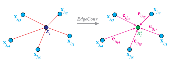
将点云表征为一个图,${\rm{G}}(V,\xi )$ ,点云的每一个点对应图中的一个结点,而图中的每一条边对应的是点之间的特征feature,称为Edge-feature。举个例子,最简单的情景,可以通过KNN来构建图。Edge Feature用$e_{ij}$来表示,定义为:
$$
e_{ij} = h_{\Theta}(x_i,x_j)
$$
$$
h_{\Theta}: {R^F} \times {R^F} \to {R^{F'}}
$$
$h_{\Theta}$是一个非线性的映射,拥有一系列可学习的参数。
提出了一个名为EdgeConv的神经网络模块Module,该模块基于卷积神经网络,可以适应在点云上的高阶任务。EdgeConv的对于第i个顶点的输出为:
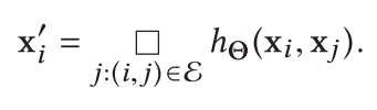
其中$□$代表的是一个对称聚合函数,如$\Sigma, max$。
可以将上述描述类比为在图像上的卷积操作。我们把$x_i$看作是中心像素点,而$x_j:(i,j) \in \xi$可以看做是围绕在点$x_i$周围的像素($x_j$事实上就是和$x_i$之间存在着feature edge的点)。所以类比这样的卷积操作,Edge-Conv可以将n个点的$F$维点云通过“卷积”转换为具有n个点的$F'$维的点云。
所以选择$h$和$□$就变得十分关键。它会直接影响EdgeConv的性能特性。
一些其他的选择在下一个小part中讨论。在本文中,作者采用的: $$ h_{\Theta}(x_i,x_j) = {\bar h}_{\Theta}(x_i, x_j - x_i) $$
从这个表达式可以非常明显的看出,既结合了全局形状结构,也结合了局部的结构信息。Global shape structure通过$x_i$捕捉,local neighborhood information通过$x_j - x_i$来捕捉。
更具体一点的说,通过如下两个公式来计算edge_feature以及x': $$ e_{ijm}' = ReLU(\theta_m \cdot(x_j - x_i) + \phi_m \cdot x_i) $$ $$ x_{im}' = \mathop {\max }\limits_{j:(i,j) \in \xi }e_{ijm}' $$
可以通过shared MLP实现。$\Theta = (\theta_1, …, \theta_M,\phi_1, …, \phi_M)$
文中采用了Dynamic Graph Update,即动态图更新。在每一层计算结束得到新的$x'$后,会根据在特征空间上的最近邻(其实就是x’间的欧式距离)关系,动态更新图。这也是该文章命名的由来。动态更新可以使得EdgeConv的感受野变得越来越大,与点云的直径一样大,同时还很稀疏。
在每一层之后,根据新的特征点云$x'$,在特征空间上的距离,对于每一个点,使用KNN寻找其k个最近点,重新构建Feature Edge。
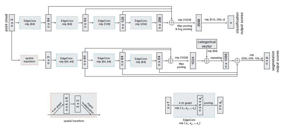
网络结构
网络结构的整体结构并不是我关注的重点。作者给出的网络结构有两个:一个用于classification,一个用于segmentation。
同时,需要说明的是,作者在Sec.4中描述的网络结构与贴的图不一致。这里采用的是修正后的网络结构图。
部分关键代码
寻找KNN,获得feature_edge的代码:
def knn(x,k):
    inner = -2 * torch.matmul(x.transpose(2, 1), x)
    xx = torch.sum(x**2, dim=1, keepdim=True)
    pairwise_distance = -xx - inner - xx.transpose(2, 1)

    idx = pairwise_distance.topk(k=k, dim=-1)[1]        #(batch_size, num_points, k)
    return idx


def get_graph_feature(x, k=20, idx=None, dim9 = False):
    # x: (batch_size, 3, num_points)
    batch_size = x.size(0)
    num_points = x.size(2)
    x = x.view(batch_size, -1, num_points)
    if idx is None:
        if dim9 == False:
            idx = knn(x, k=k)
        else:
            idx = knn(x[:, 6:], k=k)
    device = torch.device('cuda')

    idx_base = torch.arange(0, batch_size, device=device).view(-1,1,1)*num_points

    idx = idx + idx_base

    idx = idx.view(-1)

    _,num_dims,_ = x.size()

    x = x.transpose(2,1).contiguous()   # (batch_size, num_points, num_dims) --> (batch_size*num_points, num_dims)
    feature = x.view(batch_size*num_points, -1)[idx, :]     # KNN
    feature = feature.view(batch_size, num_points, k, num_dims)
    x = x.view(batch_size, num_points, 1, num_dims).repeat(1,1,k,1)

    feature = torch.cat((feature-x, x), dim=3).permute(0, 3, 1, 2).contiguous()

    return feature      # (batch_size, 2*num_dims, num_points, k)
下面这部分代码是分类网络,从中可以窥到EdgeConv以及动态更新的机制:
class DGCNN_cls(nn.Module):
    def __init__(self, args, output_channels = 40):
        super(DGCNN_cls, self).__init__()
        self.args = args
        self.k = args.k

        self.bn1 = nn.BatchNorm2d(64)
        self.bn2 = nn.BatchNorm2d(64)
        self.bn3 = nn.BatchNorm2d(128)
        self.bn4 = nn.BatchNorm2d(256)
        self.bn5 = nn.BatchNorm1d(args.emb_dims)

        self.conv1 = nn.Sequential(nn.Conv2d(6,64, kernel_size = 1, bias = False),
                                    self.bn1,
                                    nn.LeakyReLU(negative_slope=0.2))
        self.conv2 = nn.Sequential(nn.Conv2d(64*2, 64, kernel_size=1, bias = False),
                                    self.bn2,
                                    nn.LeakyReLU(negative_slope=0.2))
        self.conv3 = nn.Sequential(nn.Conv2d(64*2, 128, kernel_size=1, bias = False),
                                    self.bn3,
                                    nn.LeakyReLU(negative_slope=0.2))
        self.conv4 = nn.Sequential(nn.Conv2d(128*2, 256, kernel_size=1, bias = False),
                                    self.bn4,
                                    nn.LeakyReLU(negative_slope=0.2))
        self.conv5 = nn.Sequential(nn.Conv1d(512, args.emb_dims, kernel_size=1, bias=False),
                                    self.bn5,
                                    nn.LeakyReLU(negative_slope=0.2))
        self.linear1 = nn.Linear(args.emb_dims*2, 512, bias=False)
        self.bn6 = nn.BatchNorm1d(512)
        self.dp1 = nn.Dropout(p=args.dropout)
        self.linear2 = nn.Linear(512, 256)
        self.bn7 = nn.BatchNorm1d(256)
        self.dp2 = nn.Dropout(p=args.dropout)
        self.linear3 = nn.Linear(256, output_channels)

    def forward(self, x):
        batch_size = x.size(0)
        x = get_graph_feature(x, k=self.k)      # (batch_size, 3, num_points) --> (batch_size, 3*2, num_points, k)
        x = self.conv1(x)                       # (batch_size, 3*2, num_points, k) --> (batch_size, 64, num_points, k)
        x1 = x.max(dim=-1, keepdim=False)[0]    # (batch_size, 64, num_points, k) --> (batch_size, 64, num_points)

        x = get_graph_feature(x1, k=self.k)     # (batch_size, 64, num_points) --> (batch_size, 64*2, num_points, k)
        x = self.conv2(x)                       # (batch_size, 64*2, num_points, k) --> (batch_size, 64, num_points, k)
        x2 = x.max(dim=-1, keepdim=False)[0]    # (batch_size, 64, num_points, k) --> (batch_size, 64, num_points)

        x = get_graph_feature(x2, k=self.k)     # (batch_size, 64, num_points) --> (batch_size, 64*2, num_points, k)
        x = self.conv3(x)                       # (batch_size, 64*2, num_points, k) --> (batch_size, 128, num_points, k)
        x3 = x.max(dim=-1, keepdim=False)[0]    # (batch_size, 128, num_points, k) --> (batch_size, 128, num_points)

        x = get_graph_feature(x3, k=self.k)     # (batch_size, 128, num_points) --> (batch_size, 128*2, num_points, k)
        x = self.conv4(x)                       # (batch_size, 128*2, num_points, k) --> (batch_size, 256, num_points, k)
        x4 = x.max(dim=-1, keepdim=False)       # (batch_size, 256, num_points, k) --> (batch_size, 256, num_points)

        x = torch.cat((x1, x2, x3, x4), dim=1)  # (batch_size, 64+64+128+256, num_points)

        x = self.conv5(x)                       #(batch_size, 64+64+128+256, num_points) --> (batch_size, emb_dims, num_points)
        x1 = F.adaptive_max_pool1d(x, 1).view(batch_size, -1)           # (batch_size, emb_dims, num_points) --> (batch_size, emb_dims)
        x2 = F.adaptive_avg_pool1d(x, 1).view(batch_size, -1)           # (batch_size, emb_dims, num_points) --> (batch_size, emb_dims)
        x = torch.cat((x1, x2), 1)                                      # (batch_size, emb_dims*2)

        x = F.leaky_relu(self.bn6(self.linear1(x)), negative_slope=0.2) # (batch_size, emb_dims*2) --> (batch_size, 512)
        x = self.dp1(x)
        x = F.leaky_relu(self.bn7(self.linear2(x)), negative_slope=0.2) # (batch_size, 512) --> (batch_size, 256)
        x = self.dp2(x)
        x = self.linear3(x)                                             #(batch_size, 256) --> (batch_size, output_channels)

        return x
特性
置换不变性
考虑每一层的输出:
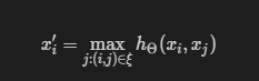
每一层的输出$x_i'$是不会随着输入$x_j$的输入顺序改变而变化的。其原因在于max是一个对称的函数。
平移不变性
EdgeConv有着部分额平移不变性。因为:
$$
h_{\Theta}(x_i,x_j) = {\bar h}_{\Theta}(x_i, x_j - x_i)
$$
从这个公式就可以看出,函数的一部分是Translation-dependent的,而另一部分是具有平移不变性的。
用EdgeConv的理论重新审视其他网络
PointNet
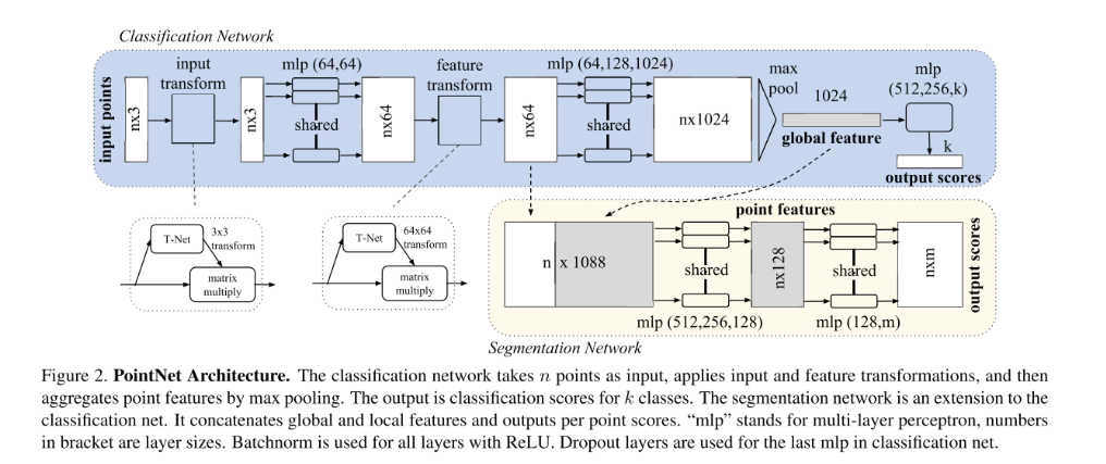 PointNet的特点是将每一个点进行单独处理,不断抽象到高维空间(这也正是其缺乏局部结构信息的缺陷来源)。
所以PointNet实际是本文理论的一种特殊情形。$k = 1, \xi = \emptyset$,采用的
PointNet的特点是将每一个点进行单独处理,不断抽象到高维空间(这也正是其缺乏局部结构信息的缺陷来源)。
所以PointNet实际是本文理论的一种特殊情形。$k = 1, \xi = \emptyset$,采用的Edge Function实际上是:$h_{\Theta}(x_i,x_j) = h_{\Theta}(x_i)$.只考虑到Global feature而忽略了local geometry。
PointNet++
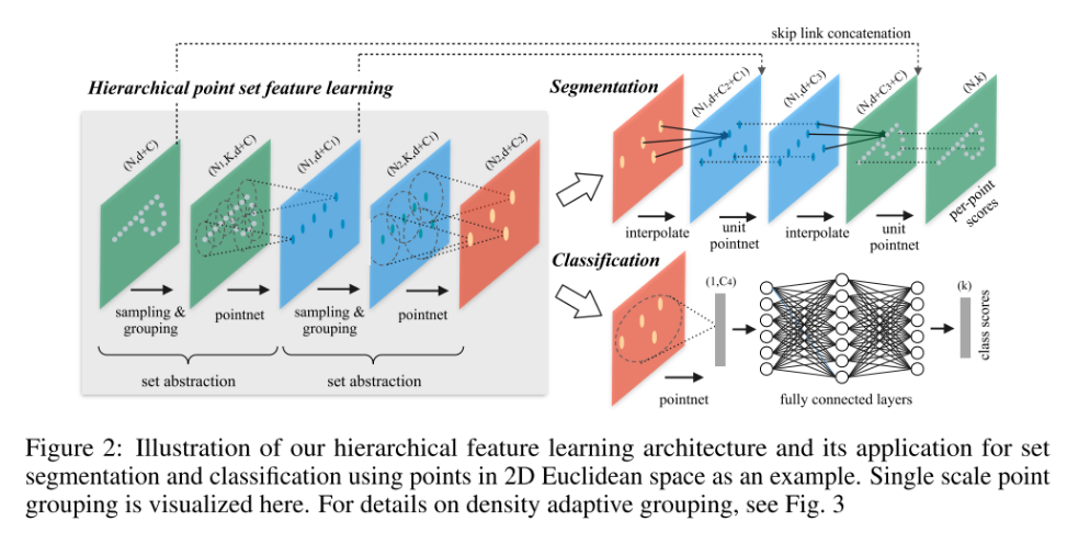 PointNet++意识到了PointNet中存在的问题,所以它通过FPS采样,然后通过
ball query构造局部点集,再通过PointNet抽象出局部特征。
PointNet++ 首先通过欧氏距离来构建图Graph,然后每经过一个layer对图进行一次粗糙化。在每一层,首先通过FPS选取一些点,只有这些被选取的点将保留,其他的点都将被抛弃。通过这种方法,图会在每经过一层网络后变得越来越小。同时,PointNet++使用输入数据的欧式距离来计算点对关系,所以就导致了他们的图在整个训练过程中是固定的,而不是动态调整的(DGCNN一大特点就是动态图)。Edge Function是$h_{\Theta}(x_i,x_j)=h_{\Theta}(x_j)$
MoNet 与 PCNN
笔者还未阅读这两篇论文。看的时候没什么概念。先留个坑。